[Math] Gradient (구배, 기울기, 경사, 경도) Vector

Gradient (구배, 기울기, 경사, 경도), $\nabla f(\textbf{x})$

Multi-Variate Function (=Scalar Field, Multi-Variable Function) $f(\textbf{x})$에서
input $\textbf{x}$의 미세한 변화에 대해 (scalar) output이
1) 가장 가파르게 증가하는 direction(방향)과
2) 그 증가하는 변화율의 정도를 magnitude(크기)로 가지는
Vector Field (Multi-Variable Vector Valued Function)를 구하는 것이
바로 Gradient $f(\textbf{x})$=$\nabla f(\textbf{x})$임.

 

Gradient를 통해,
scalar field $f(\textbf{x})$(◀ Potential Energy, Voltage, Loss Function)로부터
vector field $\nabla f(\textbf{x})$ (◀ Gravitational Field, Electric Field, Gradient)를 얻어냄.

• scalar field의 각각의 위치에서
  해당 scalar field가 가장 빠르게 증가하는 방향 (direction of steepest ascent, 최대경사의 방향) 과
  그 기울기(=증가하는 정도) 를 나타내는
  vector field를 구함.
• gradient에 -1을 곱하면, 가장 빠르게 감소하는 방향 을 가르키게 됨.

$$\nabla f (\textbf {x}) = \begin{bmatrix} \dfrac{\partial f}{\partial x_1} (\textbf{x}) \\ \vdots  \\ \dfrac{\partial f}{\partial x_n} (\textbf{x})\end{bmatrix}$$

---

예 : 3개의 component로 구성된 $\textbf{x}$를 input으로 하는 scalar field $f(\textbf{x})$에서의 gradient

해당 함수의 gradient vector field는 다음과 같음.

$$\begin{aligned}\nabla f(x,y,z)&=\left\langle \frac{\partial f(x,y,z)}{\partial x},\frac{\partial f(x,y,z)}{\partial y},\frac{\partial f(x,y,z)}{\partial z}\right\rangle \\\\ &=\frac{\partial f(x,y,z)}{\partial x}\textbf{i}+\frac{\partial f(x,y,z)}{\partial y}\textbf{j}+\frac{\partial f(x,y,z)}{\partial z}\textbf{k} \\\\ &=\begin{bmatrix} \frac{\partial f(x,y,z)}{\partial x}\\\\\frac{\partial f(x,y,z)}{\partial y}\\\\\frac{\partial f(x,y,z)}{\partial z}\end{bmatrix}\end{aligned}$$

---

Nabla (or Del) Operator

Gradient 에서 사용되는 연산자 $\nabla$는

• 해밀턴의 연산자,
• nabla,
• del 등으로 불림.

이 중 nabla와 del이라는 이름이 많이 사용됨.

nabla $\nabla$자체를 partial derivative operator들을 component로 가지는 vector로 표기(아래 참고)하기도 함.

$$\nabla =\begin{bmatrix}\frac{\partial}{\partial x}\\\\\frac{\partial}{\partial y}\\\\\frac{\partial}{\partial z}\end{bmatrix}$$

 

이 $\nabla$ Vector는 일종의 연산자로

• scalar 를 output으로 하는 함수 $\textbf{f}$에 nabla를 취해주어
• vector valued function을 얻어냄. (gradient의 차원은 gradient를 취하는 함수 $f$의 input의 차원, $\text{dim }\textbf{x}$과 같음)

Gradient에서 Nabla $\nabla$는
Function을 입출력으로 하는
일종의 Operator처럼 사용.
(scalar field ▷ vector field)

2023.06.23 - [.../Math] - [Math] Partial Derivatives (편도함수)

[Math] Partial Derivatives (편도함수)

---

참고: Directional Derivatives 와 관계.

2023.06.23 - [.../Math] - [Math] Directional Derivative (방향도함수)

[Math] Directional Derivative (방향도함수)

Directional Derivative는

• 특정 위치(input vector)에서
• 특정 방향을 나타내는 vector $\textbf{u}$의 방향으로 구해진
• scalar field $f$의 기울기(directional derivatives of $f$ with respect to $\textbf{u}$)

$f$의 기울기에 해당하는 gradient 에서
특정 방향을 나타내는 vector $\textbf{u}$ 성분이 어느 정도인지가 이 directive derivatives의 magnitude임.

(특정 방향의 vector를 x,y,z 축 성분으로 분리하는 것을 생각하면 됨.)

 

표기는 다음과 같음.

$$\frac{\partial f}{\partial \textbf{u}}=\nabla_\textbf{u}f=\textbf{u}\cdot \nabla f$$

---

Example 1

$f(\textbf{x})=e^{-x^2-y^2}$ scalar field(=multi-variable function)의 plot_surface는 다음과 같음.

이 scalar field의 contour는 다음과 같음 (level set으로 표현).

이 scalar field의 gradient는 다음과 같음.

$$\nabla f(\textbf{x})=\begin{bmatrix}\dfrac{\partial f(x,y)}{\partial x}\\\\\dfrac{\partial f(x,y)}{\partial y}\end{bmatrix}=\begin{bmatrix}- 2 x e^{- x^{2} - y^{2}}\\\\- 2 y e^{- x^{2} - y^{2}}\end{bmatrix}$$

---

관련 sympy code

from sympy.vector import gradient, CoordSys3D
import sympy as sp
 
R = CoordSys3D(' ')
 
Omega = sp.exp(-(R.x**2)-(R.y**2))
 
# Print omega
display(Omega)
 
# Print grad omega
display(gradient(Omega))

• 모든 gradient vector들은 level contour에 orthogonal (or perpendicular)임.

위의 그림 관련 code

import matplotlib.pyplot as plt
import numpy as np
 
xmin = ymin = -1.5
xmax = ymax = 1.5
sample_size = 100
 
def f(x,y):
  return np.exp(-(x**2)-(y**2))
 
def grad_f_x(x,y):
  return -2*x*np.exp(-(x**2)-(y**2))
 
def grad_f_y(x,y):
  return -2*y*np.exp(-(x**2)-(y**2))
 
x = np.linspace(xmin,xmax,sample_size)
y = np.linspace(ymin,ymax,sample_size)
X, Y = np.meshgrid(x, y)
 
Z  = f(X,Y)
GX = grad_f_x(X,Y)
GY = grad_f_y(X,Y)
 
fig = plt.figure(figsize=(10,10))
 
# ============================
# draw surface plot
ax = fig.add_subplot(2,2,1,projection = '3d')
ax.plot_surface(X, Y, Z, 
                #cmap = 'viridis',
                cmap='RdBu_r',
                )
# The azimuth is the rotation around the z-axis, 
# * 0 menas looking from +x,
# * -90 means looking form -y
#ax.azim=-90
 
# ============================
# draw contour
lev = 15
ax = fig.add_subplot(2,2,2)
cs = ax.contour(X,Y,Z, levels=lev)
plt.clabel(cs, inline=1, fontsize=10)
 
 
# =============================
# draw gradient 
ax = fig.add_subplot(2,1,2)
 
# draw contour for background
cs= ax.contour(X,Y,Z,levels=lev)
ax.clabel(cs, inline=1, fontsize=10)
cntr = ax.contourf(X,Y,Z, levels=lev, 
                   #cmap='RdBu_r'
                   )
plt.colorbar(cntr)
 
# draw gradient
ax.quiver(X[::4,::4],Y[::4,::4],GX[::4,::4],GY[::4,::4], color='red', 
           pivot='mid', units='width', scale=20, minshaft=4 )
plt.show()

---

Example 2:

$f(\textbf{x})=xe^{-x^2-y^2}$ scalar field(=multi-variable function)의 경우는 다음과 같음.

관련 sympy code

from sympy.vector import gradient, CoordSys3D
import sympy as sp
 
R = CoordSys3D(' ')
 
Omega = R.x*sp.exp(-(R.x**2)-(R.y**2))
 
# Print omega
display(Omega)
 
# Print grad omega
display(gradient(Omega))

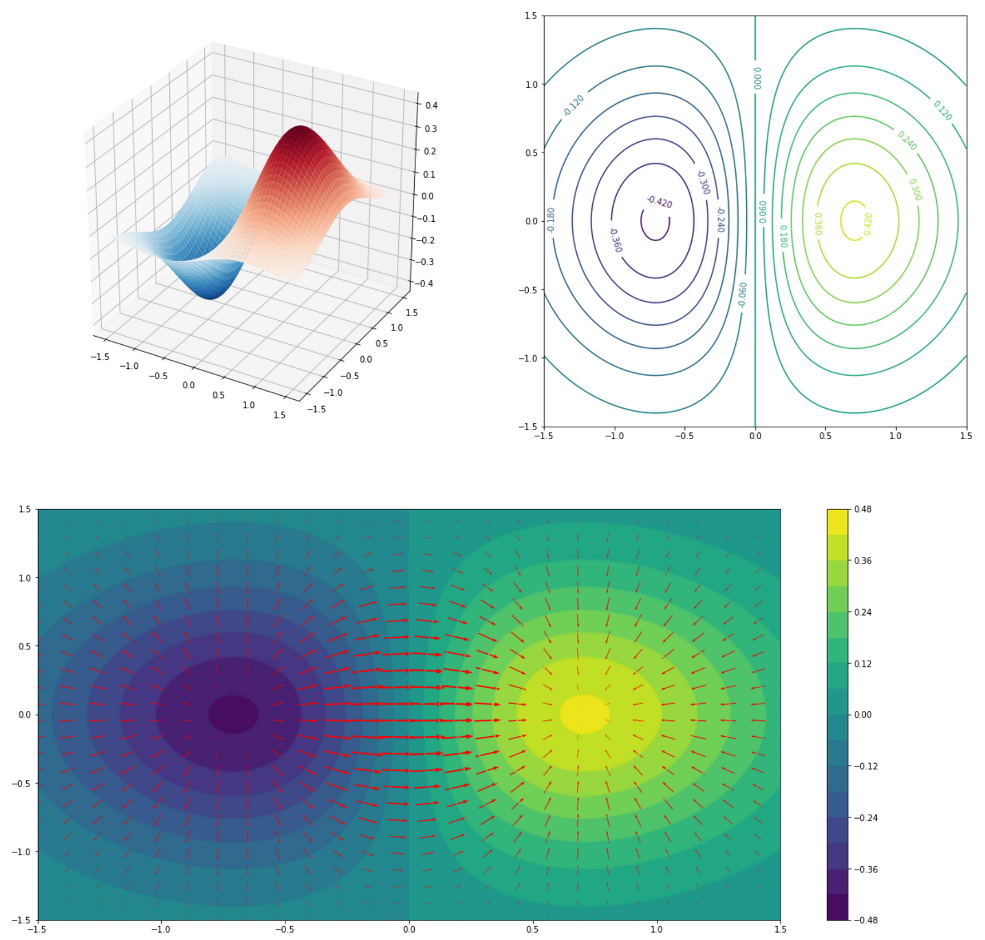
위의 그림 code

import matplotlib.pyplot as plt
import numpy as np
 
xmin = ymin = -1.5
xmax = ymax = 1.5
sample_size = 100
 
def f(x,y):
  return x*np.exp(-(x**2)-(y**2))
 
def grad_f_x(x,y):
  return -2*x**2*np.exp(-(x**2)-(y**2))+np.exp(-(x**2)-(y**2))
 
def grad_f_y(x,y):
  return -2*x*y*np.exp(-(x**2)-(y**2))
 
x = np.linspace(xmin,xmax,sample_size)
y = np.linspace(ymin,ymax,sample_size)
X, Y = np.meshgrid(x, y)
 
Z  = f(X,Y)
GX = grad_f_x(X,Y)
GY = grad_f_y(X,Y)
 
fig = plt.figure(figsize=(20,20))
 
# ============================
# draw surface plot
ax = fig.add_subplot(2,2,1,projection = '3d')
ax.plot_surface(X, Y, Z, 
                #cmap = 'viridis',
                cmap='RdBu_r',
                )
# The azimuth is the rotation around the z-axis, 
# * 0 menas looking from +x,
# * -90 means looking form -y
#ax.azim=-90
 
# ============================
# draw contour
lev = 15
ax = fig.add_subplot(2,2,2)
cs = ax.contour(X,Y,Z, levels=lev)
plt.clabel(cs, inline=1, fontsize=10)
 
 
# =============================
# draw gradient 
ax = fig.add_subplot(2,1,2)
 
# draw contour for background
cs= ax.contour(X,Y,Z,levels=lev)
ax.clabel(cs, inline=1, fontsize=10)
cntr = ax.contourf(X,Y,Z, levels=lev, 
                   #cmap='RdBu_r'
                   )
plt.colorbar(cntr)
 
# draw gradient
ax.quiver(X[::4,::4],Y[::4,::4],GX[::4,::4],GY[::4,::4], color='red', 
           pivot='mid', units='width', scale=20, minshaft=4 )
plt.show()

 

 

위 scalar field $f(\textbf{x})$ 를 gray scale의 이미지로 표현하면 다음과 같음.

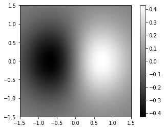
이에 대한 $\nabla f$는 다음과 같은 2개의 map (or image)로 표현된다.

 

위의 그림 code

grad = np.gradient(Z)
 
fig = plt.figure(figsize=(12,5))
 
ax = fig.add_subplot(1,2,1)
ax.set_title(r'$\frac{\partial f}{\partial \mathcal{x}}$',size=20)
grad_x=ax.imshow(grad[1],extent=[xmin,xmax,ymin,ymax],cmap = 'gray')
plt.colorbar(grad_x)
 
ax = fig.add_subplot(1,2,2)
ax.set_title(r'$\frac{\partial f}{\partial \mathcal{y}}$',size=20)
grad_y=ax.imshow(grad[0],extent=[xmin,xmax,ymin,ymax],cmap = 'gray')
plt.colorbar(grad_y)

---

Example3:

Potential Energy(위치에너지)가 $U=x^2+y^2+z^2$라고 할 때, Gravitational Field(중력장) $F=-\nabla U$를 구하라.

 

$$\begin{aligned}G&=-\nabla U\\&=-\left(\frac{\partial U}{\partial x}\textbf{i}+ \frac{\partial U}{\partial y}\textbf{j}+ \frac{\partial U}{\partial z}\textbf{k}\right)\\&=-\left[\frac{\partial}{\partial x}(x^2+y^2+z^2)\textbf{i}+ \frac{\partial}{\partial y}(x^2+y^2+z^2)\textbf{j} + \frac{\partial}{\partial z}(x^2+y^2+z^2)\textbf{k}\right]\\&=-\left[2x\textbf{i}+2y\textbf{j}+2z\textbf{k}\right]\end{aligned}$$

---

참고하면 좋은 자료

https://gist.github.com/dsaint31x/8f6d1766c9ba244b1991ff151f401af5#file-vector_gradient-ipynb

Vector_Gradient.ipynb

https://dsaint31.github.io/math/math-week03/

[Math] Week 03

---