Extended source 와 PSF

ref. Medical Imaging: Signals and Systems 2nd ed.

1. Source magnification

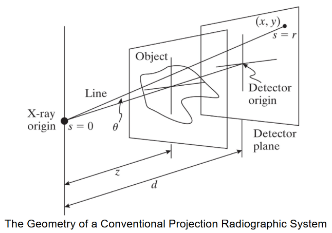
실제 X-ray source는 일정한 면적을 가진 extended source임.
Source의 서로 다른 지점에서 출발한 X-ray는 같은 point hole을 통과하더라도 detector의 서로 다른 위치에 도달함.
따라서 detector에는 source의 모양이 뒤집힌 영상 즉, inverted image 가 나타남.

 

그림 1. 같은 색의 점은 서로 대응하는 source 지점과 detector 지점을 나타냄. 그림의 Source의 붉은 점에서 출발한 X-ray는 detector의 아래쪽에 도달하는 inverted image 임.

 

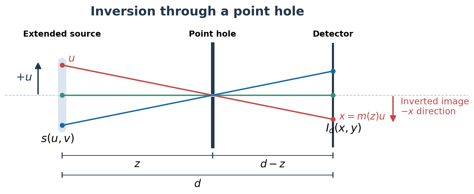
거리와 좌표는 다음과 같이 정의됨.

$$\begin{aligned}
d &: \text{source부터 detector까지의 거리} \\
z &: \text{source부터 point hole까지의 거리} \\
(u,v) &: \text{source 면의 좌표} \\
(x,y) &: \text{detector 면의 좌표}
\end{aligned}$$

Point hole이 중심축 위에 있다고 가정하면, similar triangles에 의해 다음 관계가 성립함:

$$x=-\frac{d-z}{z}u,
\qquad
y=-\frac{d-z}{z}v$$

음수 부호는 point hole을 지나면서 좌표의 방향이 반전됨을 의미(inverted image)함.

이때 source magnification (source가 ideal point가 아니기 때문에 발생하는 확대)을 다음과 같이 정의됨:

$$m(z) = -\frac{d-z}{z} = 1-\frac{d}{z}$$

따라서 source 좌표와 detector 좌표의 관계는 다음과 같음:

$$x=m(z)u, \qquad y=m(z)v $$

Point hole이 source와 detector 사이에 있어서 inverted image이므로 source magnification은 음수임.

부호는 반전 여부, 절댓값은 크기 비율을 나타냄.

 

예를 들어 source의 폭과 detector에 맺힌 source 영상의 폭은 다음 관계를 가짐.

$$D'=|m(z)|D$$

• source의 폭: D
• detector에 맺힌 source 영상의 폭: D′

Source가 point source에 가까워지면(D가 작아짐) source의 폭 자체가 작아짐.

반면 point hole이 detector에 가까워지면($z=d$) source magnification의 절댓값이 작아짐.

두 경우 모두 detector에서의 퍼짐이 감소함.

---

2. Amplitude scaling

Source 의 spatial intensity distribution은 소문자로 표기함.

$$s(u,v)$$

Detector에 나타나는 분포는 이 source의 분포 $s(u,v)$를 반전시키고 확대/축소가 이루어지고 intensity의 크기(amplitude)가 scaled 됨:

 

$$I_d(x,y)=
k s \left(
\frac{x}{m(z)} , \frac{y}{m(z)}
\right)$$

• $k$: amplitude scaling factor.
• detector의 좌표를 source magnification으로 나누어서 source distribution의 좌표를 얻어냄: 공간적 확대·축소 및 반전을 반영.

전체 신호량이 변하지 않으므로, intensity distribution이 평면검출기 상에 넓게 퍼질수록 단위 면적당 intensity는 감소해야 함.

가로와 세로가 각각 2배로 확대되면 면적은 4배가 되므로, intensity는 1/4이 됨:

그림 2. 균일한 사각형 source의 예임. 가로와 세로가 각각 절반(source magnification m=0.5)이 되면 면적은 1/4, intensity는 4배가 됨. 색은 분포의 영역을 나타내며, intensity는 아래 숫자로 표시함.

 

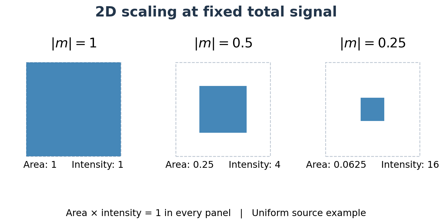
여기서는 거리 변화에 따른 전체 신호량의 변화를 무시(geometric effect에 의한 inverse square law를 무시)하면

이 관계를 다음의 적분식으로 표현할 수 있음:

 

$$\iint_{\mathbb R^2} I_d(x,y) dx dy=C$$

• $C$: 비교 과정에서 일정하게 유지하는 전체 신호량.

Detector 분포의 식을 대입하면 다음과 같음.

$$C =
k\iint_{\mathbb R^2}
s \left(
\frac{x}{m(z)} , \frac{y}{m(z)}
\right) dx dy$$

Source 좌표 $u,v$로 변수 변환함.

$$u=\frac{x}{m(z)} \qquad
v=\frac{y}{m(z)}$$

 

면적 요소의 변화는 다음과 같은 Jacobian의 determinant로 결정됨:
(Jacobian 은 u, v 의 미소 변화가 x, y 의 미소 변화로 어떻게 변환되는지를 나타냄 : $dx/du$, $dy/dv$)

$$\left|
\det
\begin{pmatrix}
m(z)&0 \\
0&m(z)
\end{pmatrix}
\right| = m^2(z)$$

2022.05.07 - [.../Math] - [Math] Jacobian : Summary

[Math] Jacobian : Summary

 

즉, 다음으로 표현 가능:

 

$$dx dy=m^2(z) du dv$$

따라서 다음이 성립함:

$$C = k m^2(z)
\iint_{\mathbb R^2}s(u,v) du dv$$

 

여기서 source distribution $s(u,v)$의 Fourier transform은 대문자로 표기함.

$$S(k_x,k_y) = \iint_{\mathbb R^2} s(u,v)e^{-j(k_xu+k_yv)} du dv$$

• 소문자 $s$: spatial intensity distribution.
• 대문자 $S$: 그 분포의 Fourier transform.
• $k_x$, $k_y$: 각 방향의 angular spatial frequency.
• $j$: imaginary unit.

Zero frequency에서는 exponential term이 1이 되므로, DC 성분은 source distribution의 전체 적분값과 같음.

$$ S(0,0) = \iint_{\mathbb R^2}s(u,v) du dv$$

 

Source distribution의 전체 적분값 $S(0,0)$ 는 source 의 방출 intensity를 적분한 값이며, detector의 전체 신호량 $C$ 는 그중 point hole을 통과하여 detector에 도달한 신호량임. 따라서 두 값을 동일하지 않음. 하지만 이들간의 비는 일정함.

 

Source distribution과 detector의 전체 신호량을 고정하면 두 값의 비율은 일정하므로,

amplitude scaling factor $k$ 는 다음과 같이 표현됨.

$$k = \frac{C}{S(0,0)} \frac{1}{m^2(z)} \propto \frac{1}{m^2(z)}$$

 

최종적으로 detector 분포는 다음과 같음.

$$\boxed{ \begin{aligned} I_d(x,y) &= k\,s \left( \frac{x}{m(z)}, \frac{y}{m(z)} \right)\\[2mm] &= \frac{C}{m^2(z)S(0,0)} s \left( \frac{x}{m(z)}, \frac{y}{m(z)} \right) \end{aligned} }$$

 

즉, amplitude scaling factor $k$는 source magnification의 제곱에 반비례하며,

source의 방출 강도가 detector 신호로 반영되는 비율 $\frac{C}{S(0,0)}$도 포함함.

---

3. Fourier transform과 delta limit

앞서 구한 detector의 intensity distribution에 Fourier transform을 적용하여,

point hole이 detector에 가까워질 때($z \to d$) 분포 $I_d(x,y)$가 어떻게 변하는지 살펴보자:

$$\begin{aligned} \mathcal F{I_d}(k_x,k_y) &= \iint_{\mathbb R^2} I_d(x,y)e^{-j(k_xx+k_yy)} dx dy \\[2mm] &= \frac{1}{m^2(z)} \iint_{\mathbb R^2} s \left( \frac{x}{m(z)}, \frac{y}{m(z)} \right) e^{-j(k_xx+k_yy)} dx dy \end{aligned}$$

 

앞서 사용한 변수변환을 다시 적용함:

$$x=m(z)u, \qquad y=m(z)v, \\ dx dy=m^2(z) du dv$$

 

그러면 amplitude scaling factor와 면적 요소의 scaling factor가 서로 상쇄됨.

$$\begin{aligned} \mathcal F\{I_d\}(k_x, k_y) &= \frac{m^2(z)}{m^2(z)} \iint_{\mathbb R^2} s(u,v) e^{-j[m(z)k_xu+m(z)k_yv]} du dv \\[2mm]
&=
S \left(m(z)k_x,m(z)k_y\right)
\end{aligned}$$

 

이것이 Fourier transform의 scaling property임.

2024.12.02 - [.../Signals and Systems] - [SS] Scaling Property (and Zero-Interpolation): Fourier Transform

[SS] Scaling Property (and Zero-Interpolation): Fourier Transform

 

공간에서 분포가 좁아지면 spatial frequency 영역에서는 분포가 넓어짐.

그림 3. Gaussian source의 예임. 왼쪽은 정규화된 2D 분포를 세로 방향으로 적분한 1D 분포이고, 오른쪽은 그 Fourier transform임. 왼쪽 곡선의 적분값은 모두 1임. Source magnification의 절댓값이 작아질수록 왼쪽은 좁아지고, 오른쪽은 넓어짐.

 

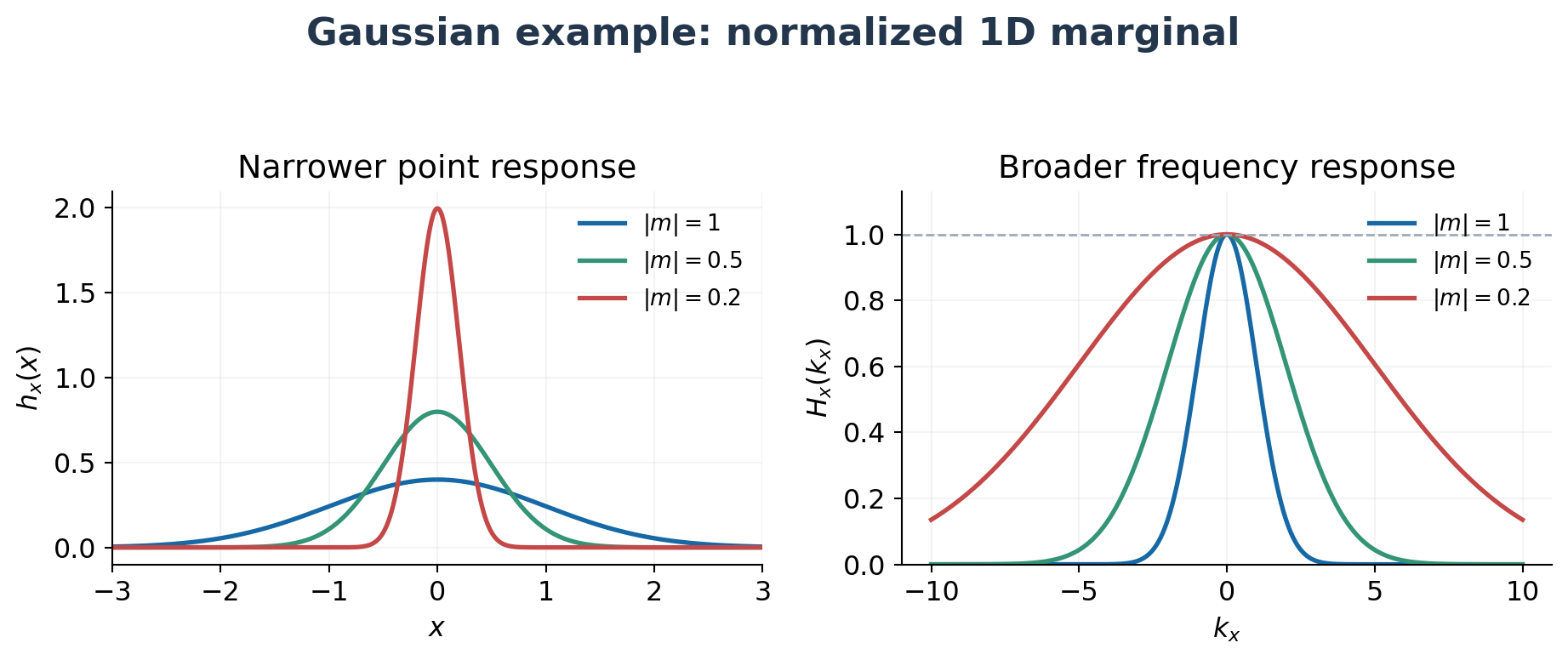
Point hole이 detector에 가까워지는 경우는 다음과 같음:

$$\lim_{z\to d}m(z) = \lim_{z\to d}\left(1-\frac{d}{z}\right) = 0$$

따라서 각각의 고정된 spatial frequency에서 Fourier transform의 값은 DC 성분에 가까워짐:

$$\lim_{z\to d}
S \left(m(z)k_x,m(z)k_y\right) = S(0,0) $$

• spatial frequency에 관계없이 같은 값을 갖는 상수에 가까워짐.

 

사용한 Fourier transform 정의에 대응하는 inverse Fourier transform은 다음과 같음:

$$I_d(x,y) = \frac{1}{(2\pi)^2}
\iint_{\mathbb R^2}
S \left(m(z)k_x, m(z)k_y\right)
e^{j(k_xx+k_yy)} dk_x dk_y$$

 

constant(상수)의 inverse Fourier transform은 delta distribution임:

$$\frac{1}{(2\pi)^2}
\iint_{\mathbb R^2}
e^{j(k_xx+k_yy)}\,dk_x dk_y =
\delta(x)\delta(y)$$

2023.10.13 - [.../Signals and Systems] - [SS] Fourier Transform of Impulse Function (Dirac Delta)

[SS] Fourier Transform of Impulse Function (Dirac Delta)

 

따라서 distribution의 의미에서 다음 극한이 성립함:

$$\boxed{
\lim_{z\to d}I_d(x,y) =
S(0,0)\delta(x,y)
}$$

• $\delta(x,y)=\delta(x)\delta(y)$

이는 $z=d$가 될수록 분포 $I_d(x,y)$의 폭이 0에 가까워지면서, 전체 적분값은 유지됨을 의미함.

즉, point hole을 detector에 가까이 두면 extended source에 의해 퍼졌던 영상이 한 점에 집중됨.

---

4. Effective PSF

Point hole은 object 면의 한 지점만 X-ray를 통과시키는 이상적인 입력으로 생각할 수 있음.

이때 detector에 나타나는 분포는 그 한 지점에 대한 system의 응답(=impulse response)임.

 

따라서 지금까지 구한 detector 분포는 extended source에 의한 point spread function, PSF의 형태를 나타냄.

전체 신호량으로 나누면 적분값이 1인 PSF가 됨.

 

$$h_d(x,y) = \frac{I_d(x,y)}{S(0,0)} \\ \boxed{h_d(x,y) = \frac{1}{m^2(z)S(0,0)} s \left( \frac{x}{m(z)}, \frac{y}{m(z)} \right)} \\ \iint_{\mathbb R^2}h_d(x,y) dx dy=1$$

 

같은 깊이에 있는 다른 object 지점도 동일한 형태로 퍼지고, detector에서 그 중심 위치만 달라진다고 가정할 경우,

Shift Invariant System을 가정하는 것임 (time으로 애기하면 이는 time invariant)

2023.08.21 - [.../Signals and Systems] - [SS] Output of LTI System : Convolution with Impulse Response

[SS] Output of LTI System : Convolution with Impulse Response

 

그러면 일반적인 영상은 각 지점에서 이동된 PSF를 신호의 크기만큼 가중하여 더한 결과 (=PSF와 convolution)임:

(LTI System에서 impulse response와 input signal의 convolution에 해당)

그림 4. 이상적인 두 선의 영상에 Gaussian 형태의 source PSF를 적용한 예임. 각 지점의 신호가 주변으로 퍼지면서 선의 경계가 흐려짐. 중앙 PSF의 밝기는 모양을 보여 주기 위해 별도로 조정됨.

 

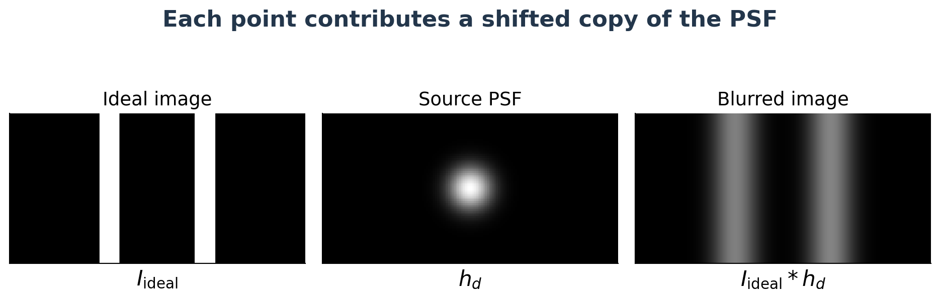
이를 적분으로 표현하면 다음과 같음.

$$I_{\mathrm{blurred}}(x,y) = \iint_{\mathbb R^2}
I_{\mathrm{ideal}}(\xi,\eta)
h_d(x-\xi,y-\eta) d\xi d\eta$$

• ideal image: point source를 가정했을 때 detector에 형성되는 영상. Object의 기하학적 확대가 이미 반영된 영상임.
• $\xi$, $\eta$: ideal image의 각 지점을 나타내는 detector 좌표.
• shifted PSF: 각 지점의 신호가 주변으로 퍼지는 분포.

이 적분은 convolution의 정의와 같음:

$$\boxed{I_{\mathrm{blurred}} = I_{\mathrm{ideal}}*h_d }$$

Point hole이 detector에 가까워지면 정규화된 PSF는 delta distribution에 가까워짐.

$$\lim_{z\to d}h_d(x,y)=\delta(x,y)$$

 

Delta와의 convolution은 원래 영상을 그대로 유지함.

$$I_{\mathrm{ideal}}*\delta = I_{\mathrm{ideal}}$$

point hole을 통해 관찰한 inverted source image는 일반적인 영상에서 각 점을 퍼뜨리는 effective PSF로 동작함.

• Object와 detector 사이의 거리를 줄이면
• 이 PSF의 폭이 감소하여, extended source에 의한 geometric blur가 줄어듦.
• 이 결과는 동일한 깊이($z$)와 shift-invariant 근사에서의 source blur에 관한 것임.

---

같이 보면 좋은 자료들

2022.10.11 - [Programming/DIP] - [DIP] Deconvolution: Richardson-Lucy deconvolution algorithm

[DIP] Deconvolution: Richardson-Lucy deconvolution algorithm

2022.09.26 - [Programming/DIP] - [DIP] Modulation Transfer Function and Contrast

[DIP] Modulation Transfer Function and Contrast

https://dsaint31.me/mkdocs_site/DIP/cv2/etc/dip_convolution/

BME

---