Homographic transformation 이란
Homographic transformation(호모그래피 변환)은
- projective transformation(투영 변환) 또는
- homography(호모그래피)라고도 불리며,
- 한 평면의 점들을 다른 평면의 점들로 매핑하는 기하학적 변환임.
이 변환은 computer vision(컴퓨터 비전), image processing(이미지 처리)에서
- image rectification(이미지 보정),
- perspective correction(원근법 수정),
- 3D reconstruction(3D 재구성) 등의 작업에 널리 사용됨.
BME228
Geometric Transformations of Images Goals Learn to apply different geometric transformation to images like translation, rotation, affine transformation etc. You will see these functions: cv2.getPerspectiveTransform Transformations Transformation 이란? T
dsaint31.me
Homographic transformation(호모그래피 변환)은
- 3x3 matrix(행렬)로 표현되며,
- homogeneous coordinates(동차 좌표계)에서 점들에 대해 작동함.
Homogeneous coordinates(동차 좌표계)에서는
Cartesian coordinates(데카르트 좌표계)의 점 (x, y)가
(x, y, 1)로 표현됨.
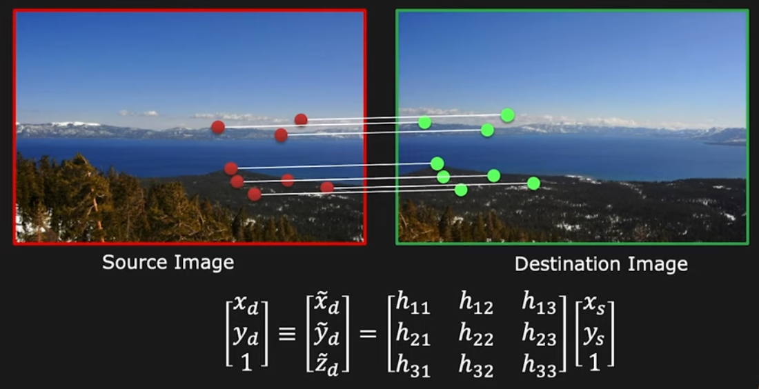
변환은 다음과 같은 방정식으로 설명됨:
$$ \begin{aligned}\begin{bmatrix} x' \\ y' \\ w' \end{bmatrix} &= \begin{bmatrix} h_{11} & h_{12} & h_{13} \\ h_{21} & h_{22} & h_{23} \\ h_{31} & h_{32} & 1 \end{bmatrix} \begin{bmatrix} x \\ y \\ 1 \end{bmatrix} \\ &= \begin{bmatrix} a_{11} & a_{12} & t_{1} \\ a_{21} & a_{22} & t_{2} \\ v_1 & v_2 & 1 \end{bmatrix}\begin{bmatrix} x\\ y \\ 1 \end{bmatrix} \\ &= \begin{bmatrix} a_{11}x+a_{12}y+t_{1} \\ a_{21}x+a_{22}y+t_{2} \\ v_1 x + v_2 y + 1\end{bmatrix} \end{aligned}$$
여기서 $(x, y)$는 원래 평면의 점, $(x', y')$는 변환된 평면의 대응 점, $w'$는 정규화 요소임.
- $\begin{bmatrix} a_{11} & a_{12} \\ a_{21} & a_{22} \end{bmatrix}$ : non singular linear matrix! (affine transform과 관련됨)
- $(t_{1}, t_{2})$ : translation.
- $v_1 x + v_2 y + 1$ : scaling factor, 이미지에서의 위치 $(x,y)$에 따라 scaling 정도가 다름.
- $v_1, v_2$ : affine transform에서는 이들은 0 이 됨.
이 matrix(행렬) $\mathbf{H}$는
- homography matrix(호모그래피 행렬)라고 불리며,
- 9개의 요소 중 하나가 1로 고정되기 때문에 8개의 자유도를 가짐.
3x3 matrix(행렬) $\mathbf{H}$는 9개의 요소를 가지고 있지만,
homogeneous coordinates(동차 좌표계)에서 정의되므로 하나의 요소를 고정해야 함.
일반적으로 matrix(행렬)의 $\mathbf{H}_{33}$ 요소를 1로 설정하여 나머지 8개의 요소에 대한 자유도를 계산함.
따라서 homography matrix(호모그래피 행렬)은 8의 DoF를 가지게 됨:
- 8개의 DoF를 구하기 위해서, 식이 8개 필요함.
- 이는 4개의 correspondances (=4개의 대응점페어) 가 있어야 구할 수 있음.
Homographic transformation의 주요 특성과 응용 분야
- Preservation of Straight Lines(직선의 보존):
- Homographic transformation(호모그래피 변환)은 직선을 직선으로 매핑함.
- 이 특성은 perspective correction(원근법 수정)과 image rectification(이미지 보정)에 유용함.
- 단, transformed line의 orientation은 원래 line의 position과 orientation에 의해 결정됨:
- 때문에 평행한 직선들은 변형 이후에는 평행이 유지되지 않음 (직선성은 보존되나...).
- 앞서 본 matrix 에서 $v_1, v_2$가 0이 아니기 때문에 position에 따라 scaling factor가 달라지고,
- 이는 transformed line의 orientation에 영향을 줌.
- 참고로, affine transform에서는 transformed line의 orientation 이 원래 line의 orientation에 의해서 결정됨. 때문에 평행성이 유지됨.
- Perspective Effects(원근 효과):
- Homography(호모그래피)는 원근 효과를 모델링할 수 있어,
- 다양한 각도에서 본 장면을 합성하거나 원근 왜곡을 수정하는 데 유용함.
- Applications in Image Stitching(이미지 스티칭):
- 파노라마 생성에서 homographies(호모그래피)는
- 서로 다른 시점에서 촬영한 여러 이미지를 정렬하고 결합하여 하나의 일관된 이미지로 만듦.
- 3D Reconstruction(3D 재구성):
- Computer vision(컴퓨터 비전)에서 homographies(호모그래피)는
- 다양한 시점에서 촬영한 여러 이미지로부터 장면의 3D 구조를 추론하는 데 사용됨.
- Camera Calibration(카메라 보정):
- Homographies(호모그래피)는
- 카메라의 intrinsic 및 extrinsic parameters를 결정하는 과정에서 사용됨.
Homography(호모그래피)를 계산하기 위해서는
원래 평면과 변환된 평면 사이의 최소 네 개의 점 대응이 필요함.
이 corresponances는 homography matrix(호모그래피 행렬)의 elements의 값을 구하는데 사용됨.
위의 matrix 의 elements 가 결국 parameters이고, 이들을 구하는 fitting을 수행하게 된다.
주로 OLS나 TLS 등을 이용하여 구할 수 있음 (Camera Calibration과 유사함).
4개 이상의 여러 correspondances를 이용하는 경우(=over determined system),
- RANSAC을 통해 noise인 outlier를 제거하고,
- Simiarlity Transform(=isotropic scaling tansform)을 통해 data normalization을 해준 후 (
- 모든 points들의 원점으로부터의 평균거리가 $\sqrt{2}$가 되도록 해주는게 일반적임)
- EVD 혹은 SVD 기반의 Least Squares Solution으로 구하면 됨.
몇가지 예
원래 평면에서 점 $(x, y)$가 $(2, 3)$이라고 가정해봄.
Homography matrix(호모그래피 행렬) $\mathbf{H}$는 다음과 같음:
$$ \mathbf{H} = \begin{bmatrix} 1 & 0 & 0 \\ 0 & 1 & 0 \\ 0 & 0 & 1 \end{bmatrix} $$
- 이 matrix(행렬)는 단위 행렬(identity matrix)이므로,
- 변환 후의 점 $(x', y', w')$는 $(2, 3, 1)$이 됨.
- 여기서 $w'$는 1이며, 이는 변환된 좌표가 정규화되었음을 의미함.
이제 scaling factor가 2인 경우를 고려해봄.
Homography matrix(호모그래피 행렬) $\mathbf{H}$는 다음과 같음:
$$ \mathbf{H} = \begin{bmatrix} 2 & 0 & 0 \\ 0 & 2 & 0 \\ 0 & 0 & 1 \end{bmatrix} $$
이 경우, 변환 후의 점 $(x', y', w')$는 다음과 같이 계산됨:
$$ \begin{bmatrix} x' \\ y' \\ w' \end{bmatrix} = \begin{bmatrix} 2 & 0 & 0 \\ 0 & 2 & 0 \\ 0 & 0 & 1 \end{bmatrix} \begin{bmatrix} 2 \\ 3 \\ 1 \end{bmatrix} = \begin{bmatrix} 4 \\ 6 \\ 1 \end{bmatrix} $$
따라서, scaling factor 가 2인 경우, 점 $(2, 3)$는 $(4, 6)$로 변환됨.
참고로 $w'$는 1로, 이는 변환된 좌표가 정규화되었음을 의미함.
즉, 이 변환에 의해 점은 원래 크기의 2배로 확대되어 보이게 됨.
the normalization factor (w') 가 다른 값을 가지는 경우:
정규화 요소 $w'$가 1이 아닌 다른 값을 가지는 경우,
변환된 좌표 $(x', y')$는 $w'$로 나누어져야 함.
예를 들어, $w'$가 2인 경우:
$$ \begin{bmatrix} x' \\ y' \\ w' \end{bmatrix} = \begin{bmatrix} h_{11} & h_{12} & h_{13} \\ h_{21} & h_{22} & h_{23} \\ h_{31} & h_{32} & 1 \end{bmatrix} \begin{bmatrix} x \\ y \\ 1 \end{bmatrix} $$
$w' =2 $ 인 경우, 변환된 좌표는 다음과 같이 정규화됨:
- $ x'_{\text{normalized}} = \frac{x'}{w'} $
- $ y'_{\text{normalized}} = \frac{y'}{w'} $
따라서, $w'$가 2인 경우, 변환된 좌표 $(4, 6)$는 ((2, 3))로 정규화됨.
이와 같이 (w')는 변환된 좌표의 스케일을 조정하는 역할을 하며, 최종적으로 정규화된 좌표를 계산하는 데 사용됨.
같이 보면 좋은 자료들
[Math] Homogeneous Coordinate and Projective Geometry
Homogeneous Coordinates (동차 좌표)와 Projective Geometry (사영 기하학):1. 개요:1-1. Homogeneous Coordinates의 정의와 특성:Homogeneous Coordinates (동차 좌표)는 Euclidean Coordinates (유클리드 좌표) 시스템을 확장하여 Pr
dsaint31.tistory.com
2024.06.16 - [.../Math] - [Math] Geometry: Euclidean, Projective, Non-Euclidean
[Math] Geometry: Euclidean, Projective, Non-Euclidean
Euclidean Geometry(유클리드 기하학), Projective Geometry(사영 기하학), Non-Euclidean Geometry(비유클리드 기하학)기하학(Geometry)은 공간과 도형의 성질을 연구하는 수학의 한 분야임.기하학은 여러 종류가 있
dsaint31.tistory.com
'Programming > DIP' 카테고리의 다른 글
| [CV] Fitting (0) | 2024.06.13 |
|---|---|
| [DIP] Image Stitching (0) | 2024.06.13 |
| cv.cornerSubPix : 코너 검출 정확도 향상 (0) | 2024.06.12 |
| [DIP] functional plot and image plot. (0) | 2024.01.21 |
| [DIP] Image Quality 관련 정량화 지표들: Resolution, Contrast, SNR (0) | 2023.10.04 |