Optical Flow: Lucas Kanade Method (LK method, 1981)
Lucas-Kanade Method은
- 특징점을 중심으로 하는 local window를 선택하여,
- 해당 window내에서 모든 pixel이 brightness constancy contraint를 만족한다는 가정 하의 linear system model을 이용하여 sparse optical flow를 구하는 알고리즘을 가리킴.
- local optimization method에 기반하다는 점에서 Horn-Shunck 메서드와 대비됨.
작은 local window를 사용하기 때문에 계산량이 작다는 장점을 가지나, large motion에 취약.
key point에 의존하며, 일반적으로 정확도 면에서 Horn-Shunck보다 떨어지는 경우가 많음.
2024.11.17 - [Programming/DIP] - [CV] Optical Flow: Horn-Schunck Method (1981)
[CV] Optical Flow: Horn-Schunck Method (1981)
Horn-Schunck(혼 슁크) 방법은Optical Flow를 구하는 기법으로Global Optimization Method임.Optical flow는 연속된 영상프레임 사이에서Global Optimization 기반으로 물체의 이동(motion vector or velocity)을 추출하는 기법
dsaint31.tistory.com
고전적인 Optical Flow Algorithm 중에서도 가장 기본적인 방법으로
Iterative Lucas-Kanade Method w/ Pyramids 등으로 발전됨
이 자료는 Shree Nayar 교수님의 Youtube 강의자료를 정리함
Lucas-Kanade Method | Optical Flow
Assumption
For each pixel, assume Motion Field, and hence Optical Flow $(u,v)$, is constant within a small neighborhood (=window, kernel) $\mathbf{W}$.
That is for all points $(k,l) \in \mathbf{W}$:
$$
\nabla_xI(k,l)u + \nabla_y I(k,l)v + \nabla_t I(k,l) = 0
$$
Brightness Constancy Constraint (=Optical Flow Constraint)가
하나의 pixel에서만 성립하던 것을,
동일한 $\mathbf{u}=\begin{bmatrix}u & v \end{bmatrix}^\top$가
window $\mathbf{W}$ 내의 모든 pixels $(k,l) \in \mathbf{W}$ 에 적용되도록 확장함.
under-determined system → over-determined system:
least squares 를 이용하여 $\mathbf{u}$를 구할 수 있음.
Lucas-Kanade Solution
For all pixels $(k,l)\in \mathbf{W}:$
$$
\nabla_x I(k,l) + \nabla_y I(k,l) = -\nabla_t I(k,l).
$$
Let the size of window $\mathbf{W}$ be $n\times n$.
Matrix Equation으로 표현하면 다음과 같음.
$$
\begin{matrix} \begin{bmatrix} \nabla_x I(1,1) & \nabla_y I(1,1) \\ \vdots & \vdots \\ \nabla_x I(k,l) & \nabla_y I(k,l) \\ \vdots & \vdots \\ \nabla_x I(n,n) & \nabla_y I(n,n) \end{bmatrix} &\begin{bmatrix} u \\ v \end{bmatrix} & = &\begin {bmatrix} -\nabla_t I(1,1) \\ \vdots\\ -\nabla_t I(k,l)\\ \vdots \\ -\nabla_t I(n,n) \end{bmatrix} \\ \mathbf{A} &\textbf{u} & = & \mathbf{b} \\ \text{known} & \text{unknown} & = & \text{known} \\ n^2 \times 2 & 2 \times 1 & = & n^2 \times 1\end{matrix}
$$
같은 windows내의 모든 pixel에 대해 같은 motion vector를 공유한다는 제한 조건을 통해서
$n^2$ equations를 얻어냄:
이를 통해 over-determined system → Least Squares Solution!!
이는 다음에 해당함.
Solve Linear System: $\mathbf{A}\mathbf{u} = \mathbf{b}$
$$
\begin{aligned}\mathbf{A}^\top \mathbf{A} \mathbf{u} &= \mathbf{A}^\top \mathbf{b} \\ \begin{bmatrix} \sum_\mathbf{W} \nabla_x I \nabla_x I & \sum_\mathbf{W} \nabla_x I \nabla_y I \\ \sum_\mathbf{W} \nabla_y I \nabla_x I & \sum_\mathbf{W} \nabla_y I \nabla_y I \end{bmatrix} \mathbf{u} &= \begin{bmatrix} -\sum_\mathbf{W} \nabla_x I \nabla_t I \\ -\sum_\mathbf{W} \nabla_y I \nabla_t I \end{bmatrix} \\ \mathbf{u}&=(\mathbf{A}^\top\mathbf{A})^{-1}\mathbf{A}^\top \mathbf{b}\end{aligned}
$$
- 위 식에서 $\sum_\mathbf{W}$ 는 Window 내에서 합을 의미함.
- 이는 각 윈도우에 동일한 가중치로 합을 구하기도 하지만, Gussian 분포를 이용한 weighted sum이 사용되는 경우가 보다 많음.
Solution Stability
$\mathbf{u}=(\mathbf{A}^\top\mathbf{A})^{-1}\mathbf{A}^\top \mathbf{b}$ 는
- OLS의 normal equation의 형태이며
- $\mathbf{A}^\top \mathbf{A}$ 가 invertible (=not singular) matrix이면서 well-conditioned 여야 solution을 구할 수 있음.
[Math] ill-posed, well-posed, ill-conditioned, well-conditioned matrix (or problem)
[Math] ill-posed, well-posed, ill-conditioned, well-conditioned matrix (or problem)
well-posed matrix and well-conditioned matrix$A\textbf{x}=\textbf{b}$와 같은 linear system에서 system matrix $A$가 invertible하다면 해당 linear system(달리 말하면 연립방정식)이 well-posed라고 할 수 있다.하지만, 해당 matrix
dsaint31.tistory.com
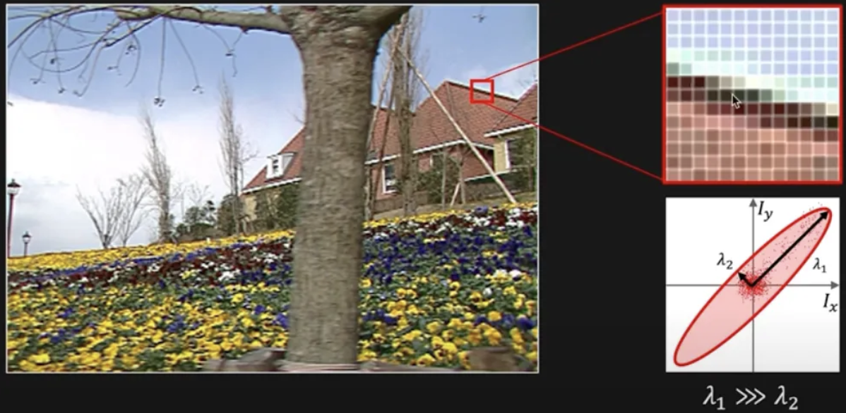
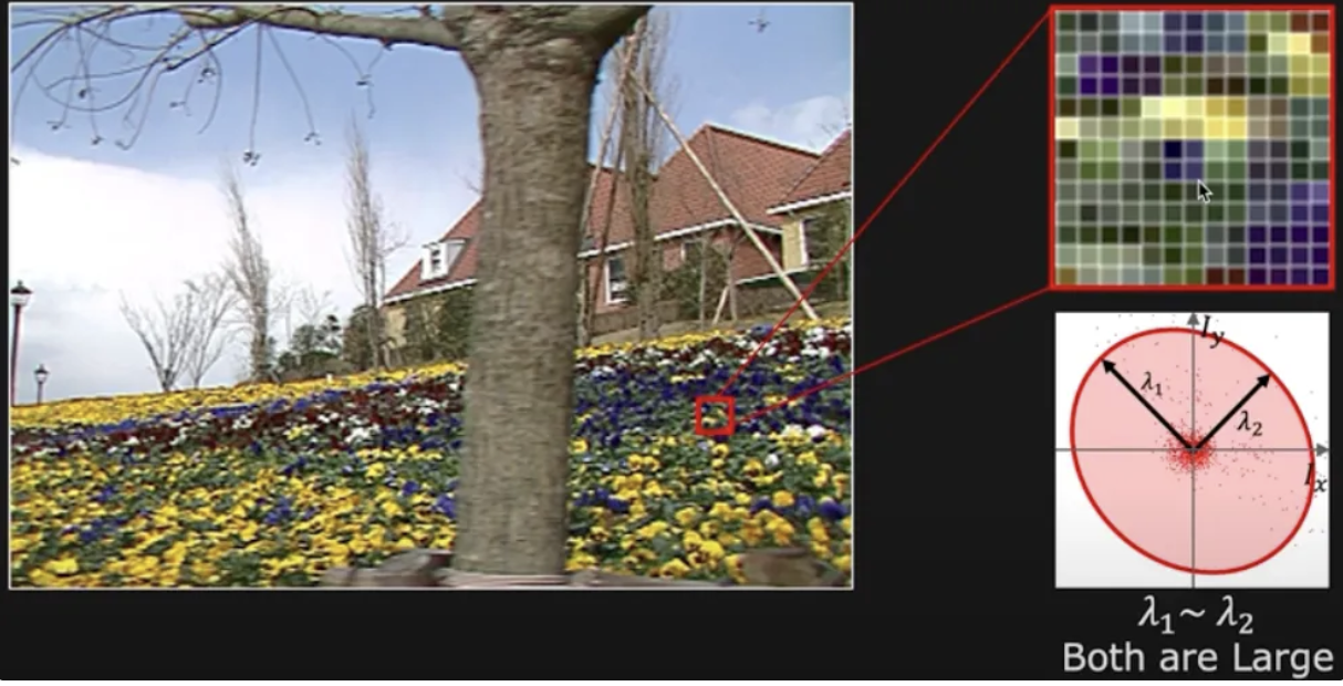
이는 $2\times 2$ matrix인 $\mathbf{A}^\top \mathbf{A}$ 의 eigen values $\lambda_1, \lambda_2$ 가 다음을 만족해야함.
- $\lambda_1 > \epsilon, \lambda_2 > \epsilon$ 로 너무 작지 않음
- $\lambda_1 \ge \lambda_2$ 이지만, 지나치게 차이가 커서는 안됨($\text{not }\lambda_1 \ggg \lambda_2$)
Condition Number $\kappa$는 다음과 같음.
$$
\kappa = \frac{\sqrt{\lambda_{\text{max}}}}{\sqrt{\lambda_{\text{min}}}}
$$
eigenvalues 를 통해 solution이 얼마나 안정적으로 구해질 수 있는지를 정리하면 다음과 같음.
- eigenvalue가 둘 다 너무 작은 경우, 분모가 작아서 Condition Number가 커지는 경우가 많아서 solution 을 reliable하게 구하기 어려움.
- eigenvalue의 차이가 클 경우도 마찬가지로 Condition Number가 매우 커짐.
- 때문에 두 eigenvalue가 적절히 둘 다 비슷하게 큰 수를 가지면서 차이가 덜한 경우 (corner에 해당) solution을 reliable하게 구할 수 있음.
각 경우에 대한 예를 들면 다음과 같음.

참고로, 위의 matrix와 eigenvalues의 관계는
고전적으로 corner를 검출하는 Harris-Stephen(1988)의 Corner Detection에서도 사용됨.
https://dsaint31.me/mkdocs_site/DIP/ch02_02_02_harris_corner/
BME228
Harris and Stephen Corner Detection (1988) C.Harris and M.Stephens. A Combined Corner and Edge Detector. Proceedings of the 4th Alvey Vision Conference: pages 147-151, 1988. 특정 point가 corner, edge인지 여부를 식별할 수 있는 방법 : local f
dsaint31.me
Limitations
- consecutive frame에서 large displacement (=large motion) 에 취약.
- fixed small window 를 사용하고,
- linearization에 기반함. (~Taylor Series Expansion을 사용하고 있으며, Constancy Constraint에 기반)
- textureless region이나 조명이 불균일한 경우 잘 동작하기 어려움.
- 복잡한 motion에서는 제대로 된 성능을 발휘하기 어려움: translation만을 가정하고 있음.
References
Lucas–Kanade method - Wikipedia
From Wikipedia, the free encyclopedia Computer vision technique for optical flow estimation In computer vision, the Lucas–Kanade method is a widely used differential method for optical flow estimation developed by Bruce D. Lucas and Takeo Kanade. It assu
en.wikipedia.org
2024.11.17 - [Programming/DIP] - [CV] Optical Flow: Horn-Schunck Method (1981)
[CV] Optical Flow: Horn-Schunck Method (1981)
Horn-Schunck(혼 슁크) 방법은Optical Flow를 구하는 기법으로Global Optimization Method임.Optical flow는 연속된 영상프레임 사이에서Global Optimization 기반으로 물체의 이동(motion vector or velocity)을 추출하는 기법
dsaint31.tistory.com
'Programming > DIP' 카테고리의 다른 글
| [OpenCV] K-Means Tree Hyper-parameters: FLANN based Matcher (1) | 2024.11.25 |
|---|---|
| [DIP] K-Means Tree: Nearest Neighbor Search (0) | 2024.11.25 |
| [CV] Optical Flow: Horn-Schunck Method (1981) (0) | 2024.11.17 |
| [CV] Least-Median of Squares Estimation (LMedS) (0) | 2024.11.16 |
| [DIP] Karhunen–Loève Transform (KLT) (1) | 2024.10.28 |